 - A SKEPTIC's GUIDE
  - A SKEPTIC's GUIDE
To generalize, we talk about a
system of N particles,15.5
each of which can only be in one of two possible
single-particle states.
A fully specified N-particle state of the system
would have the single-particle state of each individual
particle specified, and is not very interesting.
The partially specified N-particle state
with n of the particles in the first single-particle state
and the remaining (N-n) particles in the other
single-particle state can be realized in
![]() different ways, with
different ways, with
![]() given by Eq. (1).
Because there are only two possible single-particle states,
this case of
given by Eq. (1).
Because there are only two possible single-particle states,
this case of ![]() is called the binomial distribution.
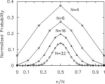
It is plotted15.6
in Fig. 15.1 for several values of N.
is called the binomial distribution.
It is plotted15.6
in Fig. 15.1 for several values of N.
 |
Note what happens to
![]() as N gets bigger:
the peak value, which always occurs at
as N gets bigger:
the peak value, which always occurs at
![]() ,
gets very large [in the plots it is compensated
by dividing by 2N, which is a big number for large N]
and the width of the distribution grows steadily
narrower - i.e. values of
,
gets very large [in the plots it is compensated
by dividing by 2N, which is a big number for large N]
and the width of the distribution grows steadily
narrower - i.e. values of
![]() far away from the peak get less and less likely
as N increases. The width is in fact the
standard deviation15.7
of a hypothetical random sample of n,
and is proportional to
far away from the peak get less and less likely
as N increases. The width is in fact the
standard deviation15.7
of a hypothetical random sample of n,
and is proportional to ![]() .
The fractional width (expressed as a fraction
of the total range of n, namely N) is therefore
proportional to
.
The fractional width (expressed as a fraction
of the total range of n, namely N) is therefore
proportional to
![]() :
: