THE UNIVERSITY OF
BRITISH COLUMBIA
PHYSICS 455
Lecture # 2 :
Wed. 8 Jan. 1997
Fundamentals
I. Statistical and Quantum Mechanics:
Historically, Statistical Mechanics (Stat Mech)
was developed before Quantum Mechanics (QM),
although the last bricks were laid in the
foundation of the former at about the same time
as the cornerstones of the latter
(namely, around the beginning of the Twentieth Century).
This makes the development of Stat Mech all the more impressive,
since Maxwell, Boltzmann and Gibbs had to work around the
conceptual problem of enumerating the infinite numbers of
states allowed in classical mechanics. Of course, QM
allows infinite numbers of states too,
in many circumstances, but it is much easier to start
with the comforting notion that the stationary states of
a quantum system are restricted to a dicsrete set of
energy levels. We (K&K and I) therefore approach
Stat Mech assuming that QM is already known and understood -
this may not be how it actually happened, but it is how it
should have happened!
II. Terminology:
- A system could be anything. We tend to try to keep it
simple, like the system composed of N helium atoms in a
box of volume V. (In this example the walls of the box
would not be considered part of the system unless explicitly
included.)
- A particle will usually be just that; but the term is used
as a quark theorist would intend it: any very simple system
all of whose properties can be exhaustively described by a small number
of quantum numbers.
- A microstate of a system is a fully specified
microscopic quantum state in which absolutely every possible
property or condition is completely specified. Unlike K&K,
I shall use the Dirac notation |
 >
to designate such a state, with the understanding that
 represents a complete set of
commuting observables for the system in question.
- A single particle quantum state is just the simplest
type of microstate. Well, actually not. One can talk about
just the spin of a single spin-˝ particle
and ignore its momentum
and other translational degrees of freedom completely, if one likes.
It's hard to get much simpler than that!
- A macrostate of a system is a partially constrained
state - one in which only certain limited aspects of its state are
specified. For example, the total energy U of the system
might be specified along with the number of particles N
of which it is composed.
- A microstate is accessible if it has the specified values
of U, N etc. That is, if it is consistent with the externally
measurable restrictions described by the macrostate's constraints.
III. The Fundamental Assumption:
Although classically every particle in a gas has a reason for being
where it is, moving with its current velocity, and so on, based on
its history of collisions etc., we have no practical way of
knowing that history and the behaviour of the particle therefore
appears random. It is disturbing (classically) to elevate that
appearance to the status of a fundamental postulate, but
that is how Stat Mech was built! With QM we have a probabilistic
interpretation of the wave function that makes the following assumption
a little more palatable, but it seems outlandish nonetheless:
"A closed system is a priori equally likely
to be found in any
one of its accessible fully specified
quantum microstates."
|
If this is true, then all of Stat Mech boils down to a problem
of enumeration: ``Let us count the ways....''
Specifically, how many different microstates are accessible,
for a given value of the macroscopic observables
like N and U?
The symbolic answer to this central question is g(N,U)
where g is called the multiplicity.
IV. An Example:
We can play around with a number of ``toy systems'' like
n cars parked in a parking lot with N spaces
or
n ``heads'' in N flips of a ``fair coin''
(one with no bias for heads or tails).
It is also fun to think about whether or not the statistical
concepts being developed here could be applied in areas
outside Physics, such as Economics; hence the somewhat frivolous
first assignment.
But the book's and my favourite model binary system
is N spin-˝ particles in a magnetic field B:
according to QM, each of these has only two choices of stationary
spin states: up ( )
or down (
 ).
How many different ways g can we have
N
 spins up and
N
 spins down for a total of N =
N
 +N
+N ?
?
By elementary arguments it is easy to show that the answer is
It is convenient to define the spin excess 2s =
N -
N
-
N ,
in terms of which
|
N! |
| g(N,s) = |
|
|
(˝N+s)! (˝N-s)! |
Using Stirling's approximation (see the Handy Math
section in Course Notes) one can approximate this exact result
by g(N,s)  g(N,0) exp(-2s2/N) for N
 1 and
s
  N.
N.

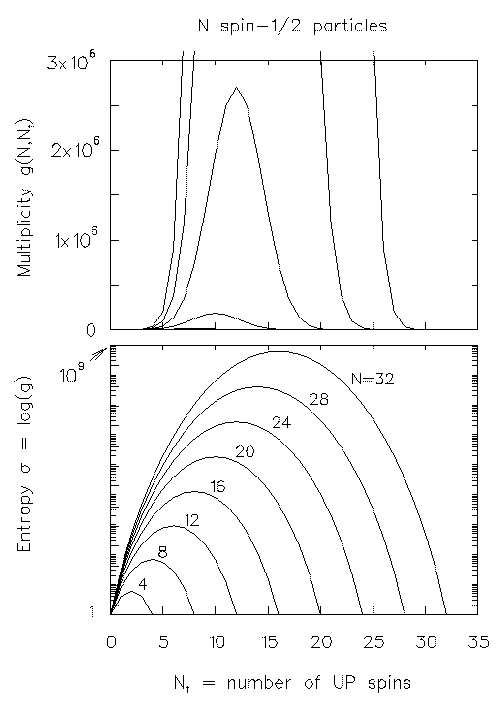
The figure above shows g(N,N )
as a function of N
 for N = 4, 8, 12, 16, 20, 24, 28 and 32, after which my computer
suffered floating-point overflow. The peak value of g is always
at N
 = N/2
and grows so rapidly with N that only on a logarithmic vertical scale
can all the curves be displayed together.
V. Entropy:
Partly for this reason (just to keep the numbers manageable)
and partly to get something that is additively
combined when we put two systems together
(as opposed to g, which is combined multiplicatively)
we prefer to use the natural logarithm of g
as the measure of the diversity of states
accessible to the system; this logarithm is called the entropy:
entropy 
 log g
= (in this case)
  o
- 2s2/N
Yes, that's what the entropy is. Just the log of the number of
accessible states.
 >
to designate such a state, with the understanding that
 represents a complete set of
commuting observables for the system in question.
 >
to designate such a state, with the understanding that
 represents a complete set of
commuting observables for the system in question.
 )
or down (
 ).
How many different ways g can we have
N
 spins up and
N
 spins down for a total of N =
N
 +N
+N ?
?
 ) =
) =  !
(N-N
 )!
)!  -
N
-
N ,
in terms of which
 g(N,0) exp(-2s2/N) for N
 1 and
s
  N.
N.

 )
as a function of N
 for N = 4, 8, 12, 16, 20, 24, 28 and 32, after which my computer
suffered floating-point overflow. The peak value of g is always
at N
 = N/2
and grows so rapidly with N that only on a logarithmic vertical scale
can all the curves be displayed together.

 log g
= (in this case)
  o
- 2s2/N